10 years ago, I asked an innocent question on Twitter.


The answers came in swiftly - Untappd was the app to use. So, a few minutes later:
In the last decade, how much beer and cider have I drunk?
I've written before about how to extract your data from Untappd using their API.
(A few notes. I don't check in to every drink - I only tend to do so if it's a new beer. Some of these are only tasters of a beer - not a full pint. This is mostly an exercise in playing with R. Visit DrinkAware if you'd like to help manage your alcohol consumption.)
Quick Stats
- 985 check ins.
- 801 unique drinks
- 3.68 average rating
- 4.93 average ABV
Graphs
Is there a correlation between how strong a drink is, and how much I like it?
R
library(jsonlite) beer_data <- read_json("untappd_data.json", simplifyVector = TRUE) abv <- beer_data$beer$beer_abv scr <- beer_data$rating_score plot(abv, scr, main="ABV vs Score", xlab="ABV", ylab="Score") abline(lm(scr~abv), col="red") # regression line (y~x)
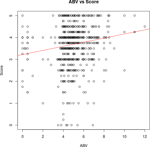
Hmmm... There's some week positive correlation there. But it's a bit muddled. Let's turn that into a hexmap:
library(hexbin) bin<-hexbin(abv, scr, xbins=10, xlab="ABV", ylab="Score") plot(bin, main="Hexagonal Binning")
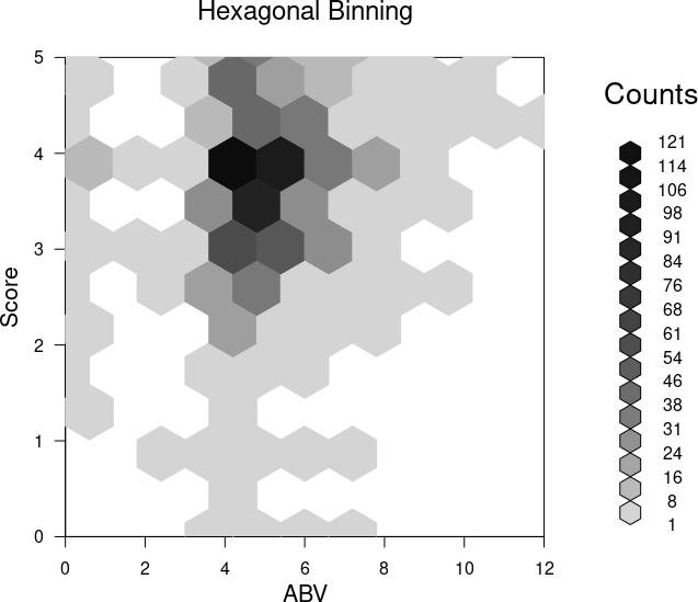
Aha! A bit easier to see. Most of the beers I drink are in the 4-5% ABV. And there is some correlation. But, mostly, I just like beer and cider. Hmmm... Which do I prefer?
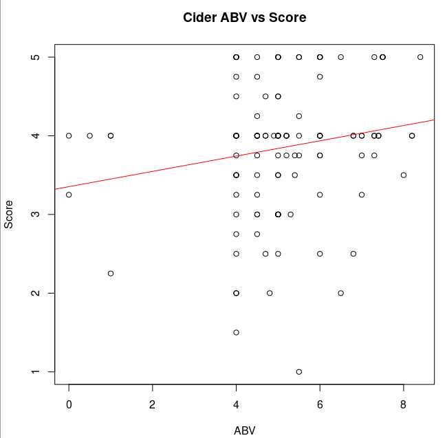
Let's take a look at Cider first:
library(data.table) beer_data <- read_json("untappd_data.json", simplifyVector = TRUE) cider <- beer_data[grepl("Cider", beer_data$beer$beer_name), ] cabv <- cider$beer$beer_abv cscr <- cider$rating_score
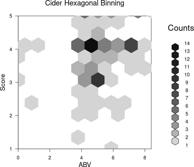
How much do I like Cider vs Beer? Just beer (OK, also includes Mead and a few other not Ciders)
justbeer <- beer_data[!grepl("Cider", beer_data$beer$beer_name), ] boxplot(cscr, ylab="Score", main="Cider Scores", ylim=c(0,5))
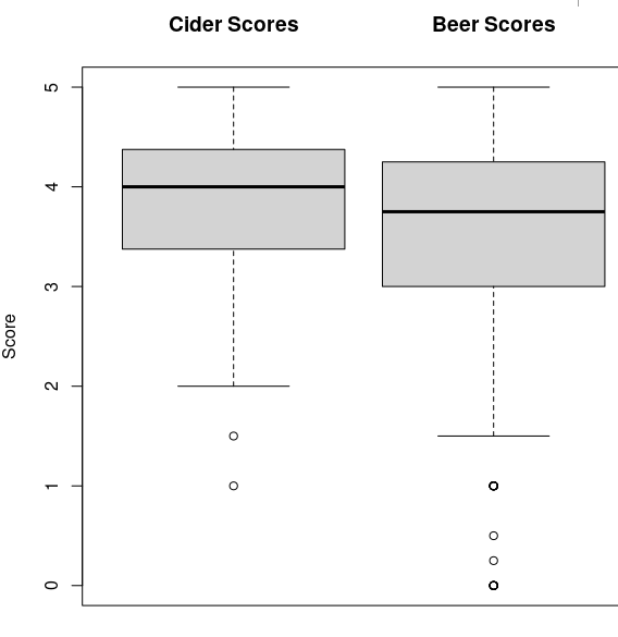
I like Cider a bit more than beer. Yup!
Let's plot that data on a map! It's a bit more complicated because the JSON is nested.
library(jsonlite) beer_data <- read_json("untappd_data.json", simplifyVector = TRUE, flatten = TRUE) venues_list <- beer_data$venue venues <- as.data.frame(do.call(rbind, venues_list)) locations_list <- venues$location locations <- as.data.frame(do.call(rbind, locations_list)) locations <-subset(locations, venue_state!="Everywhere")
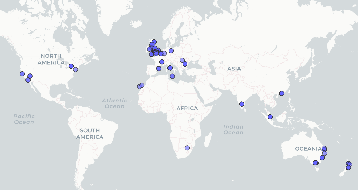
Display them on an interactive map:
library(sf) library(mapview) locations_sf <- st_as_sf(locations, coords = c("lng", "lat"), crs = 4326) mapview(locations_sf)
Let's zoom in on London:
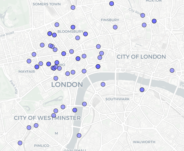
Yup! Looks about right.
Well, that was a fun afternoon of noodling with R. If you'd like to play with the data, you can download a decade of my Untappd data in JSON format